 Python在数据处理方面功能最为强大的扩展模块.
第一篇:基本数据结构介绍
一、Pandas介绍
在数据处理方面功能最为强大的扩展模块.在处理实际的金融数据时,一个条数据通常包含了多种类型的数据,例如,股票的代码是字符串,收盘价是浮点型,而成交量是整型等。在C++中可以实现为一个给定结构体作为单元的容器,如向量(vector,C++中的特定数据结构)。在Python中,pandas包含了高级的数据结构Series和DataFrame,使得在Python中处理数据变得非常方便、快速和简单。 pandas不同的版本之间存在一些不兼容性,为此,我们需要清楚使用的是哪一个版本的pandas。
import pandas as pd
pd.__version__
'0.14.1'
pandas主要的两个数据结构是Series和DataFrame,随后两节将介绍如何由其他类型的数据结构得到这两种数据结构,或者自行创建这两种数据结构,我们先导入它们以及相关模块:
import numpy as np
from pandas import Series, DataFrame
二、Pandas数据结构:Series
从一般意义上来讲,Series可以简单地被认为是一维的数组。Series和一维数组最主要的区别在于Series类型具有索引(index),可以和另一个编程中常见的数据结构哈希(Hash)联系起来。
2.1 创建Series
创建一个Series的基本格式是s = Series(data, index=index, name=name),以下给出几个创建Series的例子。首先我们从数组创建Series:
a = np.random.randn(5)
print "a is an array:"
print a
s = Series(a)
print "s is a Series:"
print s
a is an array: [-1.24962807 -0.85316907 0.13032511 -0.19088881 0.40475505] s is a Series: 0 -1.249628 1 -0.853169 2 0.130325 3 -0.190889 4 0.404755 dtype: float64
可以在创建Series时添加index,并可使用Series.index查看具体的index。需要注意的一点是,当从数组创建Series时,若指定index,那么index长度要和data的长度一致:
s = Series(np.random.randn(5), index=['a', 'b', 'c', 'd', 'e'])
print s
s.index
创建Series的另一个可选项是name,可指定Series的名称,可用Series.name访问。在随后的DataFrame中,每一列的列名在该列被单独取出来时就成了Series的名称:
s = Series(np.random.randn(5), index=['a', 'b', 'c', 'd', 'e'], name='my_series')
print s
print s.name
a -1.898245 b 0.172835 c 0.779262 d 0.289468 e -0.947995 Name: my_series, dtype: float64 my_series
Series还可以从字典(dict)创建:
d = {'a': 0., 'b': 1, 'c': 2}
print "d is a dict:"
print d
s = Series(d)
print "s is a Series:"
print s
d is a dict: {'a': 0.0, 'c': 2, 'b': 1} s is a Series: a 0 b 1 c 2 dtype: float64
让我们来看看使用字典创建Series时指定index的情形(index长度不必和字典相同):
Series(d, index=['b', 'c', 'd', 'a'])
b 1 c 2 d NaN a 0 dtype: float64
我们可以观察到两点:一是字典创建的Series,数据将按index的顺序重新排列;二是index长度可以和字典长度不一致,如果多了的话,pandas将自动为多余的index分配NaN(not a number,pandas中数据缺失的标准记号),当然index少的话就截取部分的字典内容。 如果数据就是一个单一的变量,如数字4,那么Series将重复这个变量:
Series(4., index=['a', 'b', 'c', 'd', 'e'])
a 4 b 4 c 4 d 4 e 4 dtype: float64
2.2 Series数据的访问
访问Series数据可以和数组一样使用下标,也可以像字典一样使用索引,还可以使用一些条件过滤:
s = Series(np.random.randn(10),index=['a', 'b', 'c', 'd', 'e', 'f', 'g', 'h', 'i', 'j'])
s[0]
1.4328106520571824
```Python
s[:2]
a 1.432811 b 0.120681 dtype: float64
s[['e', 'i']]
e 1.327594 i -0.634347 dtype: float64
s[s > 0.5]
a 1.432811 c 0.578146 e 1.327594 g 1.850783 dtype: float64
'e' in s
True
三、Pandas数据结构:DataFrame
在使用DataFrame之前,我们说明一下DataFrame的特性。DataFrame是将数个Series按列合并而成的二维数据结构,每一列单独取出来是一个Series,这和SQL数据库中取出的数据是很类似的。所以,按列对一个DataFrame进行处理更为方便,用户在编程时注意培养按列构建数据的思维。DataFrame的优势在于可以方便地处理不同类型的列,因此,就不要考虑如何对一个全是浮点数的DataFrame求逆之类的问题了,处理这种问题还是把数据存成NumPy的matrix类型比较便利一些。
3.1 创建DataFrame
首先来看如何从字典创建DataFrame。DataFrame是一个二维的数据结构,是多个Series的集合体。我们先创建一个值是Series的字典,并转换为DataFrame:
d = {'one': Series([1., 2., 3.], index=['a', 'b', 'c']), 'two': Series([1., 2., 3., 4.], index=['a', 'b', 'c', 'd'])}
df = DataFrame(d)
print df
one two a 1 1 b 2 2 c 3 3 d NaN 4
可以指定所需的行和列,若字典中不含有对应的元素,则置为NaN:
df = DataFrame(d, index=['r', 'd', 'a'], columns=['two', 'three'])
print df
two three r NaN NaN d 4 NaN a 1 NaN
可以使用dataframe.index和dataframe.columns来查看DataFrame的行和列,dataframe.values则以数组的形式返回DataFrame的元素:
print "DataFrame index:"
print df.index
print "DataFrame columns:"
print df.columns
print "DataFrame values:"
print df.values
DataFrame index: Index([u'alpha', u'beta', u'gamma', u'delta', u'eta'], dtype='object') DataFrame columns: Index([u'a', u'b', u'c', u'd', u'e'], dtype='object') DataFrame values: [[ 0. 0. 0. 0. 0.] [ 1. 2. 3. 4. 5.] [ 2. 4. 6. 8. 10.] [ 3. 6. 9. 12. 15.] [ 4. 8. 12. 16. 20.]]
DataFrame也可以从值是数组的字典创建,但是各个数组的长度需要相同:
d = {'one': [1., 2., 3., 4.], 'two': [4., 3., 2., 1.]}
df = DataFrame(d, index=['a', 'b', 'c', 'd'])
print df
one two a 1 4 b 2 3 c 3 2 d 4 1
值非数组时,没有这一限制,并且缺失值补成NaN:
d= [{'a': 1.6, 'b': 2}, {'a': 3, 'b': 6, 'c': 9}]
df = DataFrame(d)
print df


 a  b   c
0 1.6 2 NaN 1 3.0 6 9
在实际处理数据时,有时需要创建一个空的DataFrame,可以这么做:
df = DataFrame()
print df
Empty DataFrame Columns: [] Index: []
另一种创建DataFrame的方法十分有用,那就是使用concat函数基于Serie或者DataFrame创建一个DataFrame
a = Series(range(5))
b = Series(np.linspace(4, 20, 5))
df = pd.concat([a, b], axis=1)
print df
0 1 0 0 4 1 1 8 2 2 12 3 3 16 4 4 20
其中的axis=1表示按列进行合并,axis=0表示按行合并,并且,Series都处理成一列,所以这里如果选axis=0的话,将得到一个10×1的DataFrame。下面这个例子展示了如何按行合并DataFrame成一个大的DataFrame:
df = DataFrame()
index = ['alpha', 'beta', 'gamma', 'delta', 'eta']
for i in range(5):
    a = DataFrame([np.linspace(i, 5*i, 5)], index=[index[i]])
    df = pd.concat([df, a], axis=0)
print df


   0  1   2   3   4
alpha 0 0 0 0 0 beta 1 2 3 4 5 gamma 2 4 6 8 10 delta 3 6 9 12 15 eta 4 8 12 16 20
3.2 DataFrame数据的访问
首先,再次强调一下DataFrame是以列作为操作的基础的,全部操作都想象成先从DataFrame里取一列,再从这个Series取元素即可。可以用datafrae.column_name选取列,也可以使用dataframe[]操作选取列,我们可以马上发现前一种方法只能选取一列,而后一种方法可以选择多列。若DataFrame没有列名,[]可以使用非负整数,也就是“下标”选取列;若有列名,则必须使用列名选取,另外datafrae.column_name在没有列名的时候是无效的:
print df[1]
print type(df[1])
df.columns = ['a', 'b', 'c', 'd', 'e']
print df['b']
print type(df['b'])
print df.b
print type(df.b)
print df[['a', 'd']]
print type(df[['a', 'd']])
alpha 0 beta 2 gamma 4 delta 6 eta 8 Name: 1, dtype: float64 alpha 0 beta 2 gamma 4 delta 6 eta 8 Name: b, dtype: float64 alpha 0 beta 2 gamma 4 delta 6 eta 8 Name: b, dtype: float64 a d alpha 0 0 beta 1 4 gamma 2 8 delta 3 12 eta 4 16* * *
以上代码使用了dataframe.columns为DataFrame赋列名,并且我们看到单独取一列出来,其数据结构显示的是Series,取两列及两列以上的结果仍然是DataFrame。访问特定的元素可以如Series一样使用下标或者是索引:
print df['b'][2]
print df['b']['gamma']
4.0 4.0
若需要选取行,可以使用dataframe.iloc按下标选取,或者使用dataframe.loc按索引选取:
print df.iloc[1]
print df.loc['beta']
a 1 b 2 c 3 d 4 e 5 Name: beta, dtype: float64 a 1 b 2 c 3 d 4 e 5 Name: beta, dtype: float64
选取行还可以使用切片的方式或者是布尔类型的向量:
print "Selecting by slices:"
print df[1:3]
bool_vec = [True, False, True, True, False]
print "Selecting by boolean vector:"
print df[bool_vec]
Selecting by slices: a b c d e beta 1 2 3 4 5 gamma 2 4 6 8 10 Selecting by boolean vector: a b c d e alpha 0 0 0 0 0 gamma 2 4 6 8 10 delta 3 6 9 12 15
行列组合起来选取数据:
print df[['b', 'd']].iloc[[1, 3]]
print df.iloc[[1, 3]][['b', 'd']]
print df[['b', 'd']].loc[['beta', 'delta']]
print df.loc[['beta', 'delta']][['b', 'd']]


   b   d
beta 2 4 delta 6 12 b d beta 2 4 delta 6 12 b d beta 2 4 delta 6 12 b d beta 2 4 delta 6 12
如果不是需要访问特定行列,而只是某个特殊位置的元素的话,dataframe.at和dataframe.iat是最快的方式,它们分别用于使用索引和下标进行访问:
print df.iat[2, 3]
print df.at['gamma', 'd']
8.0 8.0
dataframe.ix可以混合使用索引和下标进行访问,唯一需要注意的地方是行列内部需要一致,不可以同时使用索引和标签访问行或者列,不然的话,将会得到意外的结果:
print df.ix['gamma', 4]
print df.ix[['delta', 'gamma'], [1, 4]]
print df.ix[[1, 2], ['b', 'e']]
print "Unwanted result:"
print df.ix[['beta', 2], ['b', 'e']]
print df.ix[[1, 2], ['b', 4]]
10.0 b e delta 6 15 gamma 4 10 b e beta 2 5 gamma 4 10 Unwanted result: b e beta 2 5 2 NaN NaN b 4 beta 2 NaN gamma 4 NaN
第二篇:快速进阶
首先,导入本篇中使用到的模块:
import numpy as np
import pandas as pd
from pandas import Series, DataFrame
一、数据创建的其他方式
数据结构的创建不止是上篇中介绍的标准形式,本篇再介绍几种。例如,我们可以创建一个以日期为元素的Series:
dates = pd.date_range('20150101', periods=5)
print dates
[2015-01-01, ..., 2015-01-05] Length: 5, Freq: D, Timezone: None
eries作为索引赋给一个DataFrame:
df = pd.DataFrame(np.random.randn(5, 4),index=dates,columns=list('ABCD'))
print df


               A         B         C         D
2015-01-01 -0.168870 0.191945 -0.906788 -1.295211 2015-01-02 -0.985849 0.312378 -1.513870 -0.876869 2015-01-03 -0.241945 1.437763 0.209494 0.061032 2015-01-04 0.139199 0.124118 -0.204801 -1.745327 2015-01-05 0.243644 -0.373126 0.333583 2.640955
只要是能转换成Series的对象,都可以用于创建DataFrame:
df2 = pd.DataFrame({ 'A' : 1., 'B': pd.Timestamp('20150214'), 'C': pd.Series(1.6,index=list(range(4)),dtype='float64'), 'D' : np.array([4] * 4, dtype='int64'), 'E' : 'hello pandas!' })
print df2
A B C D E 0 1 2015-02-14 1.6 4 hello pandas! 1 1 2015-02-14 1.6 4 hello pandas! 2 1 2015-02-14 1.6 4 hello pandas! 3 1 2015-02-14 1.6 4 hello pandas!
二、数据的查看
在多数情况下,数据并不由分析数据的人员生成,而是通过数据接口、外部文件或者其他方式获取。这里我们通过量化实验室的数据接口获取一份数据作为示例:
stock_list = ['000001.XSHE', '000002.XSHE', '000568.XSHE', '000625.XSHE', '000768.XSHE', '600028.XSHG', '600030.XSHG', '601111.XSHG', '601390.XSHG', '601998.XSHG']
raw_data = DataAPI.MktEqudGet(secID=stock_list, beginDate='20150101', endDate='20150131', pandas='1')
df = raw_data[['secID', 'tradeDate', 'secShortName', 'openPrice', 'highestPrice', 'lowestPrice', 'closePrice', 'turnoverVol']]
以上代码获取了2015年一月份全部的交易日内十支股票的日行情信息,首先我们来看一下数据的大小:
print df.shape
(200, 8)
我们可以看到有200行,表示我们获取到了200条记录,每条记录有8个字段,现在预览一下数据,dataframe.head()和dataframe.tail()可以查看数据的头五行和尾五行,若需要改变行数,可在括号内指定:
print "Head of this DataFrame:"
print df.head()
print "Tail of this DataFrame:"
print df.tail(3)
Head of this DataFrame: secID tradeDate secShortName openPrice highestPrice lowestPrice closePrice turnoverVol 0 000001.XSHE 2015-01-05 平安银行 15.99 16.28 15.60 16.02 286043643 1 000001.XSHE 2015-01-06 平安银行 15.85 16.39 15.55 15.78 216642140 2 000001.XSHE 2015-01-07 平安银行 15.56 15.83 15.30 15.48 170012067 3 000001.XSHE 2015-01-08 平安银行 15.50 15.57 14.90 14.96 140771421 4 000001.XSHE 2015-01-09 平安银行 14.90 15.87 14.71 15.08 250850023 Tail of this DataFrame: secID tradeDate secShortName openPrice highestPrice lowestPrice closePrice turnoverVol 197 601998.XSHG 2015-01-28 中信银行 7.04 7.32 6.95 7.15 163146128 198 601998.XSHG 2015-01-29 中信银行 6.97 7.05 6.90 7.01 93003445 199 601998.XSHG 2015-01-30 中信银行 7.10 7.14 6.92 6.95 68146718
dataframe.describe()提供了DataFrame中纯数值数据的统计信息:
print df.describe()


   openPrice  highestPrice  lowestPrice  closePrice   turnoverVol
count 200.00000 200.000000 200.00000 200.000000 2.000000e+02 mean 15.17095 15.634000 14.86545 15.242750 2.384811e+08 std 7.72807 7.997345 7.56136 7.772184 2.330510e+08 min 6.14000 6.170000 6.02000 6.030000 1.242183e+07 25% 8.09500 8.250000 7.98750 8.127500 7.357002e+07 50% 13.96000 14.335000 13.75500 13.925000 1.554569e+08 75% 19.95000 20.500000 19.46250 20.012500 3.358617e+08 max 36.40000 37.250000 34.68000 36.150000 1.310855e+09
对数据的排序将便利我们观察数据,DataFrame提供了两种形式的排序。一种是按行列排序,即按照索引(行名)或者列名进行排序,可调用dataframe.sort_index,指定axis=0表示按索引(行名)排序,axis=1表示按列名排序,并可指定升序或者降序:
print "Order by column names, descending:"
print df.sort_index(axis=1, ascending=False).head()
Order by column names, descending: turnoverVol tradeDate secShortName secID openPrice lowestPrice highestPrice closePrice 0 286043643 2015-01-05 平安银行 000001.XSHE 15.99 15.60 16.28 16.02 1 216642140 2015-01-06 平安银行 000001.XSHE 15.85 15.55 16.39 15.78 2 170012067 2015-01-07 平安银行 000001.XSHE 15.56 15.30 15.83 15.48 3 140771421 2015-01-08 平安银行 000001.XSHE 15.50 14.90 15.57 14.96 4 250850023 2015-01-09 平安银行 000001.XSHE 14.90 14.71 15.87 15.08
第二种排序是按值排序,可指定列名和排序方式,默认的是升序排序:
print "Order by column value, ascending:"
print df.sort(columns='tradeDate').head()
print "Order by multiple columns value:"
df = df.sort(columns=['tradeDate', 'secID'], ascending=[False, True])
print df.head()
Order by column value, ascending: secID tradeDate secShortName openPrice highestPrice lowestPrice closePrice turnoverVol 0 000001.XSHE 2015-01-05 平安银行 15.99 16.28 15.60 16.02 286043643 20 000002.XSHE 2015-01-05 万科A 14.39 15.29 14.22 14.91 656083570 40 000568.XSHE 2015-01-05 泸州老窖 20.50 21.99 20.32 21.90 59304755 60 000625.XSHE 2015-01-05 长安汽车 16.40 18.07 16.32 18.07 82087982 80 000768.XSHE 2015-01-05 中航飞机 18.76 19.88 18.41 19.33 84199357 Order by multiple columns value: secID tradeDate secShortName openPrice highestPrice lowestPrice closePrice turnoverVol 19 000001.XSHE 2015-01-30 平安银行 13.93 14.12 13.76 13.93 93011669 39 000002.XSHE 2015-01-30 万科A 13.09 13.49 12.80 13.12 209624706 59 000568.XSHE 2015-01-30 泸州老窖 19.15 19.51 19.11 19.12 14177179 79 000625.XSHE 2015-01-30 长安汽车 19.16 19.45 18.92 19.18 21233495 99 000768.XSHE 2015-01-30 中航飞机 25.38 25.65 24.28 24.60 59550293
三、数据的访问和操作
3.1 再谈数据的访问
上篇中已经介绍了使用loc、iloc、at、iat、ix以及[]访问DataFrame数据的几种方式,这里再介绍一种方法,使用":"来获取部行或者全部列:
print df.iloc[1:4][:]


      secID   tradeDate secShortName  openPrice  highestPrice  lowestPrice  closePrice  turnoverVol
39 000002.XSHE 2015-01-30 万科A 13.09 13.49 12.80 13.12 209624706 59 000568.XSHE 2015-01-30 泸州老窖 19.15 19.51 19.11 19.12 14177179 79 000625.XSHE 2015-01-30 长安汽车 19.16 19.45 18.92 19.18 21233495
我们可以扩展上篇介绍的使用布尔类型的向量获取数据的方法,可以很方便地过滤数据,例如,我们要选出收盘价在均值以上的数据:
print df[df.closePrice > df.closePrice.mean()].head()


       secID   tradeDate secShortName  openPrice  highestPrice  lowestPrice  closePrice  turnoverVol
59 000568.XSHE 2015-01-30 泸州老窖 19.15 19.51 19.11 19.12 14177179 79 000625.XSHE 2015-01-30 长安汽车 19.16 19.45 18.92 19.18 21233495 99 000768.XSHE 2015-01-30 中航飞机 25.38 25.65 24.28 24.60 59550293 139 600030.XSHG 2015-01-30 中信证券 28.50 28.72 27.78 27.86 304218245 58 000568.XSHE 2015-01-29 泸州老窖 19.04 19.23 19.00 19.15 12421826
isin()函数可方便地过滤DataFrame中的数据:
print df[df['secID'].isin(['601628.XSHG', '000001.XSHE', '600030.XSHG'])].head()
print df.shape


       secID   tradeDate secShortName  openPrice  highestPrice  lowestPrice  closePrice  turnoverVol
19 000001.XSHE 2015-01-30 平安银行 13.93 14.12 13.76 13.93 93011669 139 600030.XSHG 2015-01-30 中信证券 28.50 28.72 27.78 27.86 304218245 18 000001.XSHE 2015-01-29 平安银行 13.82 14.01 13.75 13.90 101675329 138 600030.XSHG 2015-01-29 中信证券 28.10 28.58 27.81 28.18 386310957 17 000001.XSHE 2015-01-28 平安银行 13.87 14.30 13.80 14.06 124087755 (200, 8)
3.2 处理缺失数据
在访问数据的基础上,我们可以更改数据,例如,修改某些元素为缺失值:
df['openPrice'][df['secID'] == '000001.XSHE'] = np.nan
df['highestPrice'][df['secID'] == '601111.XSHG'] = np.nan
df['lowestPrice'][df['secID'] == '601111.XSHG'] = np.nan
df['closePrice'][df['secID'] == '000002.XSHE'] = np.nan
df['turnoverVol'][df['secID'] == '601111.XSHG'] = np.nan
print df.head(10)


       secID   tradeDate secShortName  openPrice  highestPrice  lowestPrice  closePrice  turnoverVol
19 000001.XSHE 2015-01-30 平安银行 NaN 14.12 13.76 13.93 93011669 39 000002.XSHE 2015-01-30 万科A 13.09 13.49 12.80 NaN 209624706 59 000568.XSHE 2015-01-30 泸州老窖 19.15 19.51 19.11 19.12 14177179 79 000625.XSHE 2015-01-30 长安汽车 19.16 19.45 18.92 19.18 21233495 99 000768.XSHE 2015-01-30 中航飞机 25.38 25.65 24.28 24.60 59550293 119 600028.XSHG 2015-01-30 中国石化 6.14 6.17 6.02 6.03 502445638 139 600030.XSHG 2015-01-30 中信证券 28.50 28.72 27.78 27.86 304218245 159 601111.XSHG 2015-01-30 中国国航 7.92 NaN NaN 7.69 NaN 179 601390.XSHG 2015-01-30 中国中铁 8.69 8.69 8.12 8.14 352357431 199 601998.XSHG 2015-01-30 中信银行 7.10 7.14 6.92 6.95 68146718
原始数据的中很可能存在一些数据的缺失,就如同现在处理的这个样例数据一样,处理缺失数据有多种方式。通常使用dataframe.dropna(),dataframe.dropna()可以按行丢弃带有nan的数据;若指定how='all'(默认是'any'),则只在整行全部是nan时丢弃数据;若指定thresh,则表示当某行数据非缺失列数超过指定数值时才保留;要指定根据某列丢弃可以通过subset完成。
print "Data size before filtering:"
print df.shape
print "Drop all rows that have any NaN values:"
print "Data size after filtering:"
print df.dropna().shape
print df.dropna().head(10)
print "Drop only if all columns are NaN:"
print "Data size after filtering:"
print df.dropna(how='all').shape
print df.dropna(how='all').head(10)
print "Drop rows who do not have at least six values that are not NaN"
print "Data size after filtering:"
print df.dropna(thresh=6).shape
print df.dropna(thresh=6).head(10)
print "Drop only if NaN in specific column:"
print "Data size after filtering:"
print df.dropna(subset=['closePrice']).shape
print df.dropna(subset=['closePrice']).head(10)
Data size before filtering: (200, 8) Drop all rows that have any NaN values: Data size after filtering: (140, 8) secID tradeDate secShortName openPrice highestPrice lowestPrice closePrice turnoverVol 59 000568.XSHE 2015-01-30 泸州老窖 19.15 19.51 19.11 19.12 14177179 79 000625.XSHE 2015-01-30 长安汽车 19.16 19.45 18.92 19.18 21233495 99 000768.XSHE 2015-01-30 中航飞机 25.38 25.65 24.28 24.60 59550293 119 600028.XSHG 2015-01-30 中国石化 6.14 6.17 6.02 6.03 502445638 139 600030.XSHG 2015-01-30 中信证券 28.50 28.72 27.78 27.86 304218245 179 601390.XSHG 2015-01-30 中国中铁 8.69 8.69 8.12 8.14 352357431 199 601998.XSHG 2015-01-30 中信银行 7.10 7.14 6.92 6.95 68146718 58 000568.XSHE 2015-01-29 泸州老窖 19.04 19.23 19.00 19.15 12421826 78 000625.XSHE 2015-01-29 长安汽车 19.60 19.64 18.90 19.24 25546060 98 000768.XSHE 2015-01-29 中航飞机 24.65 25.63 24.53 24.98 67095945 Drop only if all columns are NaN: Data size after filtering: (200, 8) secID tradeDate secShortName openPrice highestPrice lowestPrice closePrice turnoverVol 19 000001.XSHE 2015-01-30 平安银行 NaN 14.12 13.76 13.93 93011669 39 000002.XSHE 2015-01-30 万科A 13.09 13.49 12.80 NaN 209624706 59 000568.XSHE 2015-01-30 泸州老窖 19.15 19.51 19.11 19.12 14177179 79 000625.XSHE 2015-01-30 长安汽车 19.16 19.45 18.92 19.18 21233495 99 000768.XSHE 2015-01-30 中航飞机 25.38 25.65 24.28 24.60 59550293 119 600028.XSHG 2015-01-30 中国石化 6.14 6.17 6.02 6.03 502445638 139 600030.XSHG 2015-01-30 中信证券 28.50 28.72 27.78 27.86 304218245 159 601111.XSHG 2015-01-30 中国国航 7.92 NaN NaN 7.69 NaN 179 601390.XSHG 2015-01-30 中国中铁 8.69 8.69 8.12 8.14 352357431 199 601998.XSHG 2015-01-30 中信银行 7.10 7.14 6.92 6.95 68146718 Drop rows who do not have at least six values that are not NaN Data size after filtering: (180, 8) secID tradeDate secShortName openPrice highestPrice lowestPrice closePrice turnoverVol 19 000001.XSHE 2015-01-30 平安银行 NaN 14.12 13.76 13.93 93011669 39 000002.XSHE 2015-01-30 万科A 13.09 13.49 12.80 NaN 209624706 59 000568.XSHE 2015-01-30 泸州老窖 19.15 19.51 19.11 19.12 14177179 79 000625.XSHE 2015-01-30 长安汽车 19.16 19.45 18.92 19.18 21233495 99 000768.XSHE 2015-01-30 中航飞机 25.38 25.65 24.28 24.60 59550293 119 600028.XSHG 2015-01-30 中国石化 6.14 6.17 6.02 6.03 502445638 139 600030.XSHG 2015-01-30 中信证券 28.50 28.72 27.78 27.86 304218245 179 601390.XSHG 2015-01-30 中国中铁 8.69 8.69 8.12 8.14 352357431 199 601998.XSHG 2015-01-30 中信银行 7.10 7.14 6.92 6.95 68146718 18 000001.XSHE 2015-01-29 平安银行 NaN 14.01 13.75 13.90 101675329 Drop only if NaN in specific column: Data size after filtering: (180, 8) secID tradeDate secShortName openPrice highestPrice lowestPrice closePrice turnoverVol 19 000001.XSHE 2015-01-30 平安银行 NaN 14.12 13.76 13.93 93011669 59 000568.XSHE 2015-01-30 泸州老窖 19.15 19.51 19.11 19.12 14177179 79 000625.XSHE 2015-01-30 长安汽车 19.16 19.45 18.92 19.18 21233495 99 000768.XSHE 2015-01-30 中航飞机 25.38 25.65 24.28 24.60 59550293 119 600028.XSHG 2015-01-30 中国石化 6.14 6.17 6.02 6.03 502445638 139 600030.XSHG 2015-01-30 中信证券 28.50 28.72 27.78 27.86 304218245 159 601111.XSHG 2015-01-30 中国国航 7.92 NaN NaN 7.69 NaN 179 601390.XSHG 2015-01-30 中国中铁 8.69 8.69 8.12 8.14 352357431 199 601998.XSHG 2015-01-30 中信银行 7.10 7.14 6.92 6.95 68146718 18 000001.XSHE 2015-01-29 平安银行 NaN 14.01 13.75 13.90 101675329
有数据缺失时也未必是全部丢弃,dataframe.fillna(value=value)可以指定填补缺失值的数值
print df.fillna(value=20150101).head()


      secID   tradeDate secShortName    openPrice  highestPrice  lowestPrice   closePrice  turnoverVol
19 000001.XSHE 2015-01-30 平安银行 20150101.00 14.12 13.76 13.93 93011669 39 000002.XSHE 2015-01-30 万科A 13.09 13.49 12.80 20150101.00 209624706 59 000568.XSHE 2015-01-30 泸州老窖 19.15 19.51 19.11 19.12 14177179 79 000625.XSHE 2015-01-30 长安汽车 19.16 19.45 18.92 19.18 21233495 99 000768.XSHE 2015-01-30 中航飞机 25.38 25.65 24.28 24.60 59550293
3.3 数据操作
Series和DataFrame的类函数提供了一些函数,如mean()、sum()等,指定0按列进行,指定1按行进行:
df = raw_data[['secID', 'tradeDate', 'secShortName', 'openPrice', 'highestPrice', 'lowestPrice', 'closePrice', 'turnoverVol']]
print df.mean(0)
openPrice 1.517095e+01 highestPrice 1.563400e+01 lowestPrice 1.486545e+01 closePrice 1.524275e+01 turnoverVol 2.384811e+08 dtype: float64
value_counts函数可以方便地统计频数:
print df['closePrice'].value_counts().head()
6.58 3 13.12 2 9.13 2 8.58 2 6.93 2 dtype: int64
在panda中,Series可以调用map函数来对每个元素应用一个函数,DataFrame可以调用apply函数对每一列(行)应用一个函数,applymap对每个元素应用一个函数。这里面的函数可以是用户自定义的一个lambda函数,也可以是已有的其他函数。下例展示了将收盘价调整到[0, 1]区间:
print df[['closePrice']].apply(lambda x: (x - x.min()) / (x.max() - x.min())).head()
closePrice 0 0.331673 1 0.323705 2 0.313745 3 0.296481 4 0.300465
使用append可以在Series后添加元素,以及在DataFrame尾部添加一行:
dat1 = df[['secID', 'tradeDate', 'closePrice']].head()
dat2 = df[['secID', 'tradeDate', 'closePrice']].iloc[2]
print "Before appending:"
print dat1
dat = dat1.append(dat2, ignore_index=True)
print "After appending:"
print dat
Before appending: secID tradeDate closePrice 0 000001.XSHE 2015-01-05 16.02 1 000001.XSHE 2015-01-06 15.78 2 000001.XSHE 2015-01-07 15.48 3 000001.XSHE 2015-01-08 14.96 4 000001.XSHE 2015-01-09 15.08 After appending: secID tradeDate closePrice 0 000001.XSHE 2015-01-05 16.02 1 000001.XSHE 2015-01-06 15.78 2 000001.XSHE 2015-01-07 15.48 3 000001.XSHE 2015-01-08 14.96 4 000001.XSHE 2015-01-09 15.08 5 000001.XSHE 2015-01-07 15.48
DataFrame可以像在SQL中一样进行合并,在上篇中,我们介绍了使用concat函数创建DataFrame,这就是一种合并的方式。另外一种方式使用merge函数,需要指定依照哪些列进行合并,下例展示了如何根据security ID和交易日合并数据:
dat1 = df[['secID', 'tradeDate', 'closePrice']]
dat2 = df[['secID', 'tradeDate', 'turnoverVol']]
dat = dat1.merge(dat2, on=['secID', 'tradeDate'])
print "The first DataFrame:"
print dat1.head()
print "The second DataFrame:"
print dat2.head()
print "Merged DataFrame:"
print dat.head()
The first DataFrame: secID tradeDate closePrice 0 000001.XSHE 2015-01-05 16.02 1 000001.XSHE 2015-01-06 15.78 2 000001.XSHE 2015-01-07 15.48 3 000001.XSHE 2015-01-08 14.96 4 000001.XSHE 2015-01-09 15.08 The second DataFrame: secID tradeDate turnoverVol 0 000001.XSHE 2015-01-05 286043643 1 000001.XSHE 2015-01-06 216642140 2 000001.XSHE 2015-01-07 170012067 3 000001.XSHE 2015-01-08 140771421 4 000001.XSHE 2015-01-09 250850023 Merged DataFrame: secID tradeDate closePrice turnoverVol 0 000001.XSHE 2015-01-05 16.02 286043643 1 000001.XSHE 2015-01-06 15.78 216642140 2 000001.XSHE 2015-01-07 15.48 170012067 3 000001.XSHE 2015-01-08 14.96 140771421 4 000001.XSHE 2015-01-09 15.08 250850023
DataFrame另一个强大的函数是groupby,可以十分方便地对数据分组处理,我们对2015年一月内十支股票的开盘价,最高价,最低价,收盘价和成交量求平均值:
df_grp = df.groupby('secID')
grp_mean = df_grp.mean()
print grp_mean


         openPrice  highestPrice  lowestPrice  closePrice  turnoverVol
secID 000001.XSHE 14.6550 14.9840 14.4330 14.6650 154710615 000002.XSHE 13.3815 13.7530 13.0575 13.4100 277459431 000568.XSHE 19.7220 20.1015 19.4990 19.7935 29199107 000625.XSHE 19.4915 20.2275 19.1040 19.7170 42633332 000768.XSHE 22.4345 23.4625 21.8830 22.6905 92781199 600028.XSHG 6.6060 6.7885 6.4715 6.6240 531966632 600030.XSHG 31.1505 32.0825 30.4950 31.2325 611544509 601111.XSHG 8.4320 8.6520 8.2330 8.4505 104143358 601390.XSHG 8.4060 8.6625 8.2005 8.4100 362831455 601998.XSHG 7.4305 7.6260 7.2780 7.4345 177541066
如果希望取每只股票的最新数据,应该怎么操作呢?drop_duplicates可以实现这个功能,首先对数据按日期排序,再按security ID去重:
df2 = df.sort(columns=['secID', 'tradeDate'], ascending=[True, False])
print df2.drop_duplicates(subset='secID')


       secID   tradeDate secShortName  openPrice  highestPrice  lowestPrice  closePrice  turnoverVol
19 000001.XSHE 2015-01-30 平安银行 13.93 14.12 13.76 13.93 93011669 39 000002.XSHE 2015-01-30 万科A 13.09 13.49 12.80 13.12 209624706 59 000568.XSHE 2015-01-30 泸州老窖 19.15 19.51 19.11 19.12 14177179 79 000625.XSHE 2015-01-30 长安汽车 19.16 19.45 18.92 19.18 21233495 99 000768.XSHE 2015-01-30 中航飞机 25.38 25.65 24.28 24.60 59550293 119 600028.XSHG 2015-01-30 中国石化 6.14 6.17 6.02 6.03 502445638 139 600030.XSHG 2015-01-30 中信证券 28.50 28.72 27.78 27.86 304218245 159 601111.XSHG 2015-01-30 中国国航 7.92 8.03 7.65 7.69 61877792 179 601390.XSHG 2015-01-30 中国中铁 8.69 8.69 8.12 8.14 352357431 199 601998.XSHG 2015-01-30 中信银行 7.10 7.14 6.92 6.95 68146718
若想要保留最老的数据,可以在降序排列后取最后一个记录,通过指定take_last=True(默认值为False,取第一条记录)可以实现:
print df2.drop_duplicates(subset='secID', take_last=True)


       secID   tradeDate secShortName  openPrice  highestPrice  lowestPrice  closePrice  turnoverVol
0 000001.XSHE 2015-01-05 平安银行 15.99 16.28 15.60 16.02 286043643 20 000002.XSHE 2015-01-05 万科A 14.39 15.29 14.22 14.91 656083570 40 000568.XSHE 2015-01-05 泸州老窖 20.50 21.99 20.32 21.90 59304755 60 000625.XSHE 2015-01-05 长安汽车 16.40 18.07 16.32 18.07 82087982 80 000768.XSHE 2015-01-05 中航飞机 18.76 19.88 18.41 19.33 84199357 100 600028.XSHG 2015-01-05 中国石化 6.59 7.14 6.45 7.14 1186499645 120 600030.XSHG 2015-01-05 中信证券 33.90 35.25 33.01 34.66 698627215 140 601111.XSHG 2015-01-05 中国国航 7.98 8.62 7.98 8.62 231611758 160 601390.XSHG 2015-01-05 中国中铁 9.37 9.37 8.90 9.13 469902172 180 601998.XSHG 2015-01-05 中信银行 8.15 8.33 7.91 8.16 337368242
四、数据可视化
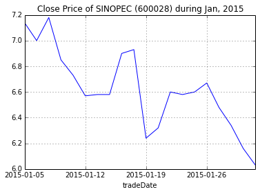
pandas数据直接可以绘图查看,下例中我们采用中国石化一月的收盘价进行绘图,其中set_index('tradeDate')['closePrice']表示将DataFrame的'tradeDate'这一列作为索引,将'closePrice'这一列作为Series的值,返回一个Series对象,随后调用plot函数绘图,更多的参数可以在matplotlib的文档中查看。
dat = df[df['secID'] == '600028.XSHG'].set_index('tradeDate')['closePrice']
dat.plot(title="Close Price of SINOPEC (600028) during Jan, 2015")
\<matplotlib.axes.AxesSubplot at 0x49b6510>